Analysis

In this section we describe a simple analytic model of both AFF and static address allocation. The goal is to develop a model that will predict the efficiency of AFF compared to a static address allocation. Our model is not sufficiently general to predict the performance in all possible scenarios, but it does provide a basis for comparison between the two architectures.

A model of AFF

The first step in our analysis is to define a simple efficiency metric. Our metric is essentially the ``cost-benefit ratio'' of transmitting bits:

$$E = \frac{\text{Useful Bits Received}}{\text{Total Bits Transmitted}}$$ (1)

In our model, bits are transmitted in packets, each of which is made up of a header and data. The cost of a packet is the cost of transmitting both its header and data. The header is not considered inherently useful, but rather something that facilitates the transmission of potentially useful data.

Every packet is part of a transaction. We assume that the transaction density, $T$, is the average number of concurrent transactions visible at any single point in the network. A limitation of our model is that the single parameter $T$ is not sufficient to describe all possible scenarios--two long transactions will have different collision characteristics than a long transaction competing with a series of short transactions, even though $T=2$ in both cases. In order to simplify our analysis, at the expense of making our model less general, we will assume that every transaction spans the same amount of time.

In our model, a packet header consists of solely a transaction identifier. At the core of our model is the assumption that a transaction is successful (that is, useful) if and only if the source uses an identifier that is unique with respect to all other transactions at the same point in the network for the entire duration of the transaction. Transactions that fail due to identifier collisions reduce efficiency because the cost of transmitted bits is incurred without the benefit of the reception of useful bits.

In the case of static allocation, where every node is given a distinct address, we assume that identifier collisions (and, therefore, failed transactions) are impossible. If, on average, we transmit $D$ bits of data with an $H$-bit header (address), the efficiency is simply:

$$E_{static} = \frac{D}{D + H}$$ (2)

Equation 2 expresses the ratio of data bits to total bits for an entire transaction, not just a single packet.

In our address-free architecture, successful transactions are no longer guaranteed. Transactions only have some probability of success due to possible identifier collisions. We assume that the entire transaction will either succeed or fail, causing either the reception or loss of all its constituent packets. Keeping in mind our assumption that all transactions are the same length, we arrive at a different efficiency metric:

$$E_{aff} = \frac{D \times P(\text{Success})} {D + H}$$ (3)

The probability of a successful transaction given in Equation 3 is dependent on three factors. The first is the the number of concurrent transactions $T$ that are contending for identifiers. Based on our previous assumption that all transactions are the same length, each transaction will overlap with the beginning or end of $2(T-1)$ other transactions in the worst case. The second factor is the size of the space from which the identifiers are drawn, $2^H$ for an $H$-bit identifier. The third factor is the algorithm used for selecting the identifiers. Heuristics for reducing the probability of identifier collisions were described in Section 3. However, we will analyze the simplest and most pessimistic scenario in which every node picks its transaction identifiers uniformly from the identifier space without regard to any learned state. This makes the analysis straightforward because each node's identifier selections are independent:

$$P( ) = \left(1 - \frac{1}{2^H}\right)^{2(T-1)}$$ (4)

Equation 4 is useful in that it gives a reasonable upper bound on the expected probability of identifier collisions. Heuristics such as listening can improve significantly on this bound in practice, as we will show in Section 5. It can be seen in Equation 3 that a significant increase in the probability of successful transactions leads directly to a significant increase in the efficiency of AFF.

Comparison of AFF to static allocation

We now wish to use our model to compare AFF over a range of identifier sizes with static allocation. In doing so we must first decide on a reasonable number of bits that should be used in static allocation for the purposes of comparison.

We assume that sensor networks will consist of tens of thousands of nodes. If addresses are assigned optimally, about 16 bits will be sufficient to address the entire network. On the other hand, past experience has shown that optimal address allocation is often difficult to achieve, or undesirable because it makes decentralized allocation difficult. The 48-bit address used in Ethernet is designed for distributed assignment of a single, universal address space. It is also meant to be sufficient for the total number of devices that exist, even though the number of nodes that make up any specific Ethernet network is much smaller. Hardware in sensor networks may be given similar global addresses--perhaps with an even larger address space given the expected scale and density of their deployment. However, to be conservative in our analysis, we will also compare AFF to 32-bit static addresses.

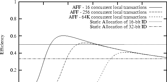
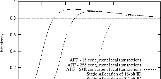
Figure 1 compares static allocation of 16- and 32-bit identifiers to AFF over a range of identifier sizes.

Figure 1: Efficiency of AFF vs. static allocation for 16-bit data.

In this example, the size of the data is 16 bits. Three different scenarios are considered for AFF: cases where 16, 256, and 65,536 transactions are simultaneously visible to individual nodes in the network. The total number of concurrent transactions in the entire network may be much larger and is not part of the model.

In the static case, transmitting 16 bits of data with a 16- or 32-bit identifier always leads to a constant 50% or 33% efficiency, respectively. These cases are represented by the flat lines in the figure. The curves describing AFF also have a consistent shape. If the number of identifier bits is too small, efficiency is low due to a large number of identifier collisions. As the number of identifier bits increases, the probability of identifier collisions quickly drops close to zero and the efficiency is dominated by the ratio of data bits to total bits (as in Equation 2). The peak of the curve represents the optimal balance between two opposing goals: minimizing the number of collisions and minimizing the number of header bits transmitted per data bit.

In a sensor network with tens of thousands of nodes, there might be only tens or hundreds of simultaneous transactions visible at any one place at any one time. Our model quantifies the intuition that AFF is more efficient if this locality of transactions allows AFF to user fewer bits than static allocation. In other words, AFF can be more efficient if locality causes a global address space to be underutilized. For example, as shown in Figure 1, AFF works optimally with only 9 identifier bits in a network where there are an average of 16 simultaneous transactions seen by any node. This is more efficient than a static assignment that might need 16 or 32 bits. On the other hand, in an extreme (and, we believe, very unlikely) case of 64K simultaneous transactions seen by every node in a 64K node network, there is no room for AFF to improve; a 16-bit address space can be fully (indeed, optimally) utilized.

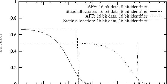
Figure 2 shows the same analysis assuming 128 bit data rather than 16.

Figure 2: Efficiency of AFF vs. static allocation for 128-bit data.

There are a number of interesting features to note. First, the larger data size makes static allocation more efficient because the same number of address bits are now being amortized over a larger number of data bits. Second, the optimal number of bits used for the AFF identifier increases. Intuitively, this is because the larger data size makes the cost of a collision higher; the increased cost of transmitting more identifier bits is worth the benefit of a lower collision rate.

Advantages of AFF

AFF is fundamentally different from static address allocation because the size of AFF's identifier space is tied to the transaction density of the network, as opposed to static allocation whose space is commensurate with the total size of the network. A node using AFF needs to select an identifier that is unique with respect to its local neighbors; the potentially large network that lies beyond a node's limited point of view becomes immaterial. AFF can take advantage of spatial and temporal locality to use fewer identifier bits than would be required for a static, globally unique allocation.

Figure 1 shows one benefit of this difference. Based on our assumptions of reasonable numbers of network densities and sizes, AFF works optimally with only 9 bits while static allocation needs 16 or 32. When amortized over only 16 bits of data, AFF can result in a increase in efficiency and thus network lifetime.

In Figure 2, which assumes larger data, the differences are less pronounced. At this design point, the efficiency of AFF and static allocation are not significantly different. However, using AFF still buys us vastly better scaling properties. As the network grows, AFF's optimum identifier size will remain the same. In contrast, the size of identifiers for globally unique static allocation must grow with the size of the network.

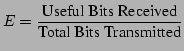
Clearly, AFF does not help in networks that do not exhibit locality. If the optimum number of bits needed by AFF is the same as the number of bits required for globally unique static allocation, traditional static allocation will always be better. This point is illustrated in Figure 3. The figure shows our model from a different perspective, describing how efficiency of the network changes as the load on it increases.

Figure 3: Efficiency of AFF vs. static allocation for 16-bit data.

Statically assigned identifiers have constant efficiency until the address space is exhausted, after which the efficiency is undefined. AFF does work beyond this point, though networks should never be so severely underprovisioned by design.

Does fewer bits mean less energy?

We have mentioned that energy savings are one of the primary motivations for using shorter identifiers. However, the actual energy savings achieved by reducing the number of bits transmitted is highly dependent on details of the radio hardware and MAC protocol in use. While 20 bits saved by AFF may have a large impact on efficiency in the user-data portion of a packet (as seen in Figure 1's example), that savings becomes meaningless if used with a MAC layer such as 802.11 that adds hundreds of bits of overhead per packet. In the higher-powered regime of laptops running complex MAC protocols, AFF makes little sense.

However, these few bits do become much more meaningful in the context of the very low-powered radios designed for sensor networks--such as those made by Radiometrix, RF Monolithics, and perhaps even the forthcoming Bluetooth radios. These radios have extremely simple MACs and framing that leads to a more direct correlation between the amount of user data sent to the radio and the energy expended to send it. Quantifying this relationship is a subject of our ongoing research.

These lower-powered radios are also often associated with limited frame sizes. The Radiometrix RPC radio, for example, can transmit only 27 bytes per frame. AFF originally came from a desire to squeeze as much information as possible into these small frames.