Corridor Traversal

Our corridor traversal algorithm assumes that the robot is traveling clockwise around a cyclic corridor. It can not detect such a corridor; it assumes that its initial position and direction are somewhere on its desired path. The shape of the corridor is assumed to be convex (modulo slight deviations such as closed doors), but has no other constraints. Although our sample environment in Figure 1 is a simple rectangular corridor, our controller will work equally well in buildings whose corners are not rectilinear.

Our controller for implementing this task is purely reactive: it contains no state and, indeed, does very little processing at all. It makes a continuous stream of instantaneous control decisions based on its current sonar state. Each of the Pioneer's seven sonars are first classified into one of three states: NEAR (an object sensed at 2m or less); MID (an object sensed between 2-5m); and FAR (an object is sensed at 5m or more).

The essence of the controller is shown in Figure 2, where the desired steady-state of each of the robots' seven front- and side-looking sonars are shown.

Figure 2: Desired steady state of all seven sonar sensors for proper direction control in a clockwise traversal of a cyclic corridor. The sonars are numbered clockwise from 0 to 6.

To maintain this state, the controller has two independent, reactive control pathways: one for speed control and one for direction control. Although implemented as a simple series of ``if-then'' clauses, these control elements are written in the ``style'' of classic behavior-based controllers. That is, they each have multiple and potentially conflicting goals that have a defined priority in their ability to affect the final control decision.

Turning Behaviors

The algorithm that governs turning is shown in Program Fragment 1.

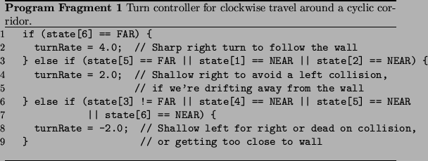
The first turning rule states that we should follow the corridor after the right-hand wall has suddenly disappeared--i.e., is no longer visible to the right side-looking sonar. In this case, where we assume we need to turn quickly to make a corner, we make a sharp (4 radian/sec) right turn.

In the case when we see a collision in one of our two left-front sensors, we make a shallow turn to the right. We also make this shallow right turn if we have drifted far enough away from the right wall that Sonar 5 can no longer see it. Note that this is less drastic action than the sharp turn taken if Sonar 6 loses sight of the wall.

Finally, we make a shallow turn to the left if we see a collision with something dead ahead or to our right (Sonars 3, 4 and 5, respectively), or if Sonar 6 indicates we are getting too close to the right wall. The dead-ahead looking sonar assumes that any detected object is a collision. In contrast, the diagonal sonars only assume a collision in the NEAR state; they normally pick up the corridor walls in the MID state, even when the robot is correctly positioned.

Speed Behaviors

Program Fragment 2 shows the code used for controlling the robot's speed.

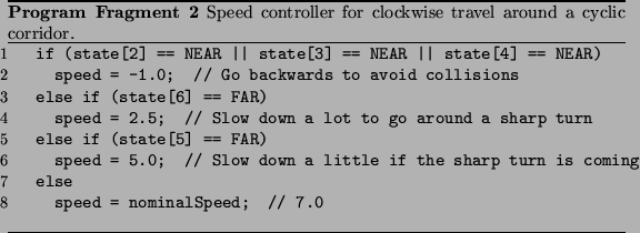
In the absence of any special conditions, it commands the robot to travel at speed nominalSpeed. This speed is normally 7.0 m/s for a leader robot, and is variable for a following robot, as will be described later.

The first special case considered is a collision. If a robot detects a very nearby object with any of its three front-looking sonars (Sonars 3, 4, and 5), it immediately backs up slowly¹ with a speed of -1.0 m/s.

Next, the robot attempts to guess when it may have a sharp turn in its future. If Sonar 5 loses sight of the wall, the controller guesses that a corner is approaching, and slows down to $^2/_3$ of its nominal speed.

Finally, if the robot thinks it is required to perform a sharp turn to the right at a corner, it further slows to $^1/_3$ of its nominal speed.

Corridor Following Results

This simple controller is surprisingly robust and reliable. Figure 3 shows plots of a robot's traverse through our SAL model.

Figure 3: a) (left) Plot of a single robot's traverse once around the corridor. Hash marks are at constant time intervals; the robot can be seen slowing down as it approaches a sharp turn. b) (right) A plot of many laps around the corridor. The robot's actions are relatively consistent.

a)

b)

It makes tight turns quite reliably, follows a reasonably straight path down the corridor despite the irregular sonar readings caused by doorways, and never loses track of the wall. The tight turns and rare loss of path around corners appears to be largely due to the robot's tendency to slow down as it approaches corners. Even after thousands of laps, the controller continues to function without failure.

Figure 4 shows the same traverse in the presence of three stationary obstacles.

Figure 4: a) (left) Plot of a single robot's traverse once around the corridor in the presence of three stationary obstacles. The robot avoids them in ways that look surprisingly ``intelligent.'' b) (right) Many laps around the corridor.

a)

b)

Again, the controller is quite robust, avoiding the vast majority of obstacles. However, it is admittedly possible to place obstacles in certain pathological ways such that the robot gets stuck and makes no further progress.