Constant Distance Following

With a good corridor following behavior, the constant distance following problem actually becomes much easier. Constrained by their corridor following, both robots can be thought of as following a simple one-dimensional path. The follower's problem has now been reduced to estimating its distance to the leader and adjusting its relative speed accordingly. The problem essentially has only one degree of freedom: speed control.

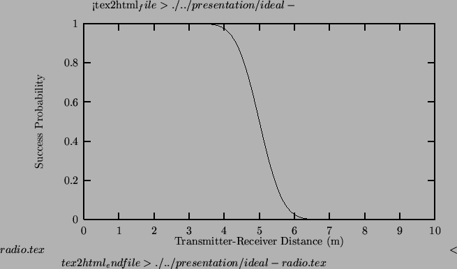
The difficulty now lies in the distance estimation. In this experiment, the follower estimates its distance from the leader by listening to a radio beacon emitted by the leader. The beacon comes from a simulated radio whose nominal transmission radius, 5m, is also the desired following distance. We model the simplest possible characteristics of Radiometrix RPC radios, where the probability of a successful packet transmission drops off sharply as the distance between the sender and receiver passes the radio's nominal transmission radius. Figure 5 shows an idealized picture of this property.

Figure 5: Idealized radio model for a radio with a nominal transmission radius of 5m.

Given this kind of radio, it seems relatively straightforward to build a controller for constant distance following. The leader sends a continuous stream of packets at a constant frequency. The follower then listens to this packet stream. Because the follower knows the leader's sending frequency, it can easily determine its packet loss rate averaged over some window of recent transmissions. 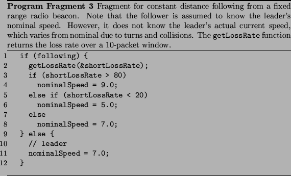A high loss rate means the leader is too far away; a low loss rate means the leader is too close. The follower can then adjust its nominal speed accordingly. Our controller that implements this policy is shown in Program Fragment 3.

The Radio Model

This brings us to the heart of our study. The success of the controller described above is, of course, critically dependent on the actual radio propagation model. A radio system that differs significantly in its behavior from the ideal shown in Figure 5 will break a controller that assumes the ideal. If we want a radio-based controller designed in simulation to work in the real world, the simulated radio must have the same behavior as a real one, to whatever level of detail is used by the controller. It is this point, in my opinion, that makes imprecise simulations possible in robotics and not in pure networking research: network controllers extract much more detailed information from the world.

Radio propogation is notoriously hard to model in many domains. Indoor models are particularly bad, where multipath interference, reflections, shadowing, and other effects are caused by a very complex environment. The success rate of a packet is extremely difficult to predict unless the transmitter-receiver distance is well within the transmitter's nominal transmission radius. As this radius is reached, the success of a transmission decreases; however, there can be islands of good reception in a sea of bad loss.

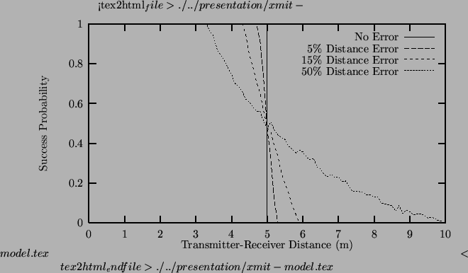
We attempt to simulate this property using an `` $(r +$   percent-error$)^2$'' radio propagation model. In this model, the success of a packet is 1 if the distance from the transmitter to the receiver is below the sender's transmission radius, 0 otherwise. However, a random error is added to or subtracted from the distance before the thresholding decision is made. The error is uniformly selected from a range that is proportional to the distance; for example, $r^\prime = r \pm 25\%$.

We studied our controller using four different percent-error settings in our simple radio model, as illustrated in Figure 6.

Figure: The `` $(r +$   percent-error$)^2$'' radio transmission model used for the robotic simulation. Four settings for the percentage error were used: 0%, 5%, 15% and 50% (from vertical to diagonal, respectively).

Zero error corresponds to a ``better-than-ideal'' model, where the success probability drops instantaneously from 1 to 0. This could theoretically allow a follower to get a fix on its desired distance to the leader with arbitrary position in a simulator, but could never be achieved in the real world due to the vagaries of real radio propagation. Five and 15 percent errors correspond more closely to the idealized real-world model shown in Figure 5 and are probably similar to real outdoor propagation conditions. 50 percent error is a pathological case where any given packet's success is unlikely to correlate well with the transmitter-receiver distance, as in an indoor environment.

Constant Distance Following Results

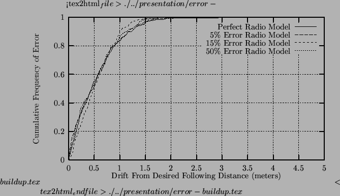
The complete controller as described in previous sections was run for each of the four radio models shown in Figure 6. For each model, a leader and follower robot were both started at opposite sides of the SAL corridor. In each case, the follower gradually caught up to the leader, and eventually settled into its steady state of continuous speed corrections in an attempt to maintain constant distance.

After this equilibrium was reached, we recorded the exact robot positions as reported by the simulator at 0.1 second intervals through 20 laps through the SAL corridor. At each time interval, we computed the difference between the desired following distance of 5m and the actual (simulated) distance between the robots. The cumulative error frequencies are shown in Figure 7.

Figure 7: Cumulative distribution of errors in following distance for the four radio models.